The space of LLM learning curves
2023-11-29
The mean test loss of LLMs scales smoothly, often approximately as a
power law as a function of model parameters, data, or training steps.
The mean loss is averaged across a large number of tokens in a corpus. But language is quite diverse. Predicting some
tokens correctly may require entirely different knowledge or skills than are required to predict other tokens. So how does the
mean loss of LLMs decompose? Are all the different pieces of knowledge or skill needed
to predict different tokens acquired smoothly, in the same way that the mean loss decreases smoothly? Or are they
acquired at different times and rates, with the mean loss curve averaging over many curves which individually look quite
different from the mean?
This question is relevant for testing different
models of neural scaling, for understanding how
predictable the capabilties
of future models will be, and broadly for just having a better picture of how neural networks learn. This post simply
provides interactive visualizations for viewing many different LLM learning curves. It is merely exploratory, and
not on its own a rigorous test of any particular hypothesis. We can still notice some interesting facts and patterns.
Below you should seen an interactive plot with three panes. The top left
pane allows you to select a token from a language corpus. The top right
pane will then show an LLM's loss on that token over many checkpoints
of training. The bottom pane displays the token, with some context, that the loss was computed
on, highlighted in red.
Wait several seconds then refresh the page if the plot doesn't appear below.
It may take multiple tries, and you may have to wait for 5-10 seconds. The app is running on a small node, and cannot
handle many simultaneous connections.
There are 10659 tokens & curves in this visualization. These are spread across
the first 20k documents of the test set of The Pile corpus.
The LLM was pythia-410m,
trained by Eleuther AI on the train set of The Pile. I forwarded the first 1024 tokens
of each document through the model, yielding at most 1023 loss values per document. Enumerating these
loss values, I simply selected token number 0, 1000, 2000, ..., so the samples are roughly uniformly
distributed across the corpus. pythia-410m is part of the Pythia family of models.
These models are trained with a learning rate warmup lasting 1% of the training run,
so the first 1430 steps. Checkpoints are at steps
0, 1, 2, 4, 8, ... 512 and then 1000, 2000, ..., 143000. We use a log scale when plotting
the curves since most movement happens very early in training, which would be almost invisible
on a linear scale. Also, some
models of neural scaling suggest
that the time scale on which different things are learned by the model might span multiple orders of magnitude.
Note that the combination of the log scale and the warmup may exaggerate the sharpness of some of the
drops in the loss.
The scatter plot on the top left pane is a UMAP projection of the training
curves. We weighted the distance function according to the density of the
checkpoints on a log scale, so that curves which are visually similar on our
plot are put close together in the projection. I'll emphasize that this projection
is based only on the loss curves, not directly on any information about what token
was being predicted or what tokens were in the context for each sample.
Some observations

There is a disconnected cluster of samples on the bottom right of the figure.
For all of these samples, we find that the loss drops extremely early in training,
and that all samples involve predicting the newline token. In fact, they involve predicting a newline
after either a period "." or a separate newline token "⏎". Note that the newline token is
the most commonly occuring token in the corpus, representing ~4.4% of tokens, and that the (⏎, ⏎) and
(., ⏎) bigrams are the most commonly occuring bigrams in the corpus, representing 1.26% and 0.74% of all
bigrams, respectively.

There is a small cluster of points above and to the right of the bulk. These samples all
involve predicting an "s" token after the apostrphe token "’". This is the 10th most
common bigram in the corpus, representing 0.16% of all bigrams.
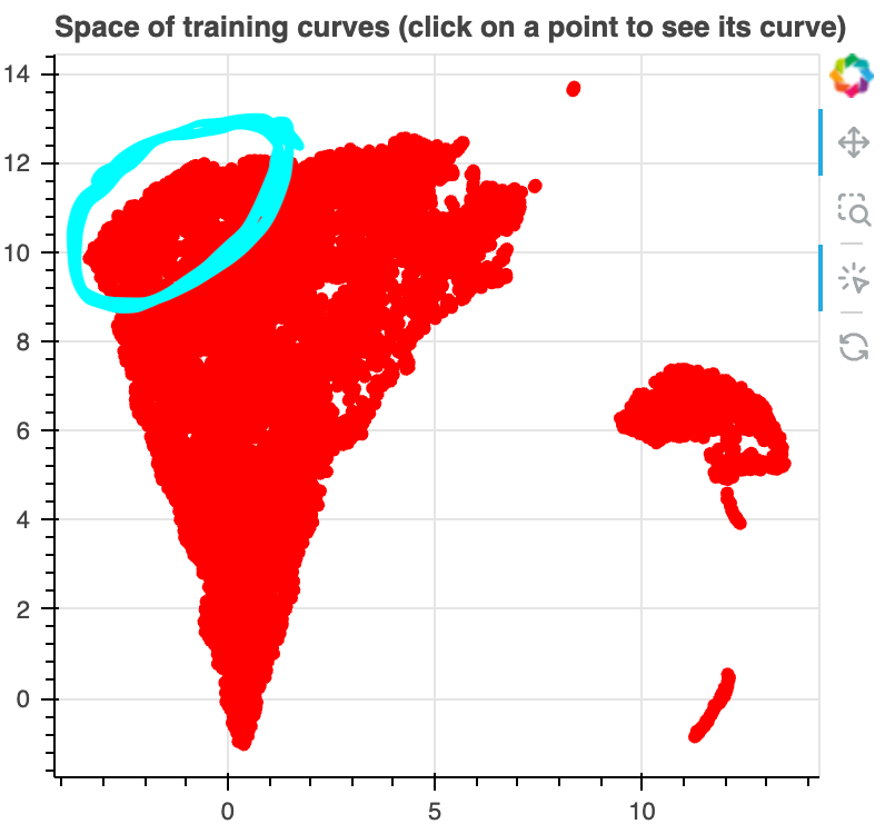
Around the upper boundary of the bulk, we find many loss curves that drop sharply early in
training. Many of these, especially at the top left of the bulk, involve predicting a token that
is part of a subsequence that occurred earlier in the context (c.f. induction heads).
Generally, as we move along the top of the bulk from right to left and then down the left side of the bulk, we
see loss curves which drop sharply later and later in training.
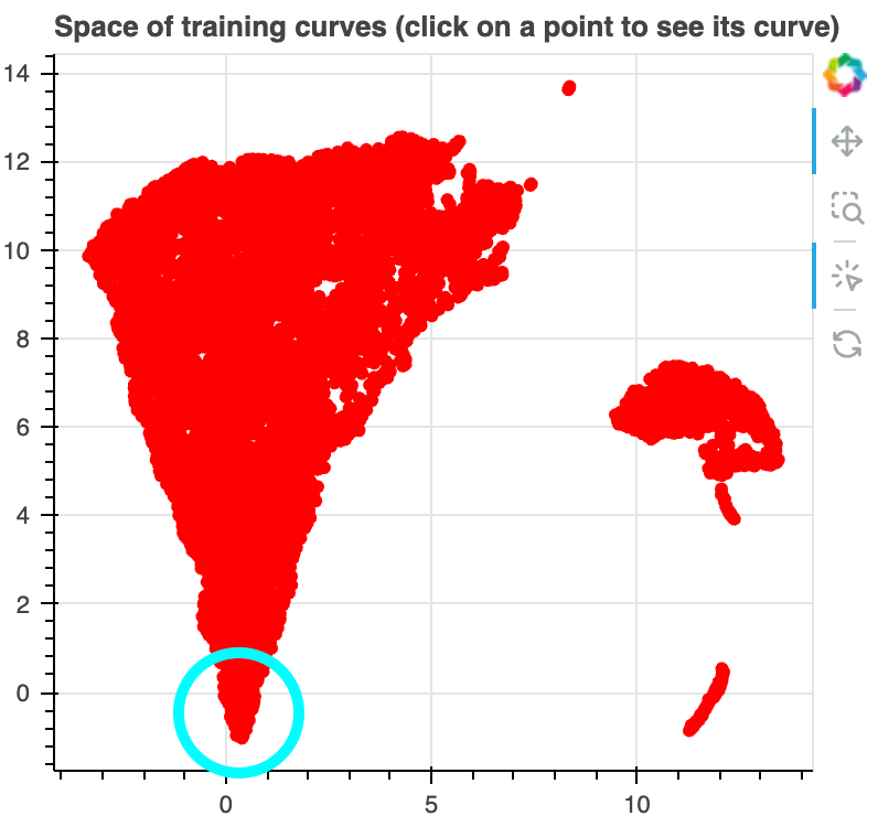
At the bottom of the bulk, we find samples where loss increases over training,
an example of inverse scaling.
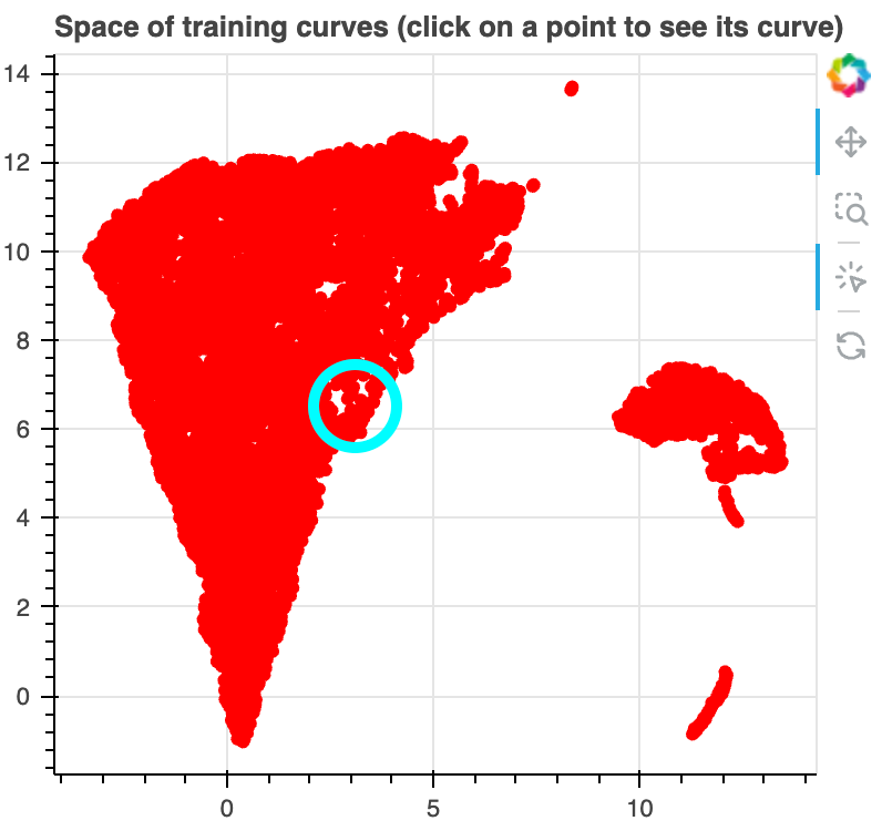
At the middle of the right side of the bulk, we find some samples where the loss
decreases and then increases. This is sort of like U-shaped scaling
(except the opposite since here
lower is better).
Variation across seeds is minimal
We see that there are many loss curves on individual tokens whose behavior is pretty far from
the mean loss curve. An important question is whether this is
due to randomness. Perhaps for each
token there is some wide distribution over possible loss curves, whose mean is similar to the mean loss across tokens. To test this, we visualize
loss curves for the "pythia-160m" model, for which we have checkpoints for four different training runs with different seeds.
Note that the models were still trained on the
same data in the same order, so the seeds just determine the initialization of the network:
Overall it seems like there is surprisingly little variation between seeds. Loss curves which deviate
substantially from the mean often do so in the same way across seeds.
Variation across model scale
Let's now look at how the loss curves for models of different size compare:
Loss curves for models of different size seem typically pretty similar. Especially for tokens where the loss
drops sharply early in training. This similarity, across seeds and model scales, is perhaps suggestive of a kind
of universality in what what and how different LLMs learn.
You can run these visualizations locally with: https://github.com/ejmichaud/llm-curve-visualization
Thanks to Davis Brown for helpful suggestions and feedback on this site and the figures. Many thanks also to Uzay Girit, Lauro Langosco, and Robert Kirk for early discussions and explorations of phase changes during LLM training.
Edited 2023-11-30: added release date to top and slightly changed some phrasing.