Understanding grokking in terms of representation learning dynamics

This post is based on the preprint Towards Understanding Grokking: An Effective Theory of Representation Learning, by Ziming Liu, Ouail Kitouni, Niklas Nolte, Eric J. Michaud, Max Tegmark, and Mike Williams. It aims to be a bit easier to read than the full paper and also includes some videos and additional discussion. It was written by Eric, with videos created by Ouail.

You are seeing v1 of this post, last updated 2022-06-18. It could change over time as we continue to think about grokking.

Last year, some researchers at OpenAI released a short paper called Grokking: Generalization Beyond Overfitting on Small Algorithmic Datasets. In this paper, they documented a curious phenomenon where their neural networks would generalize long after overfitting their training dataset. 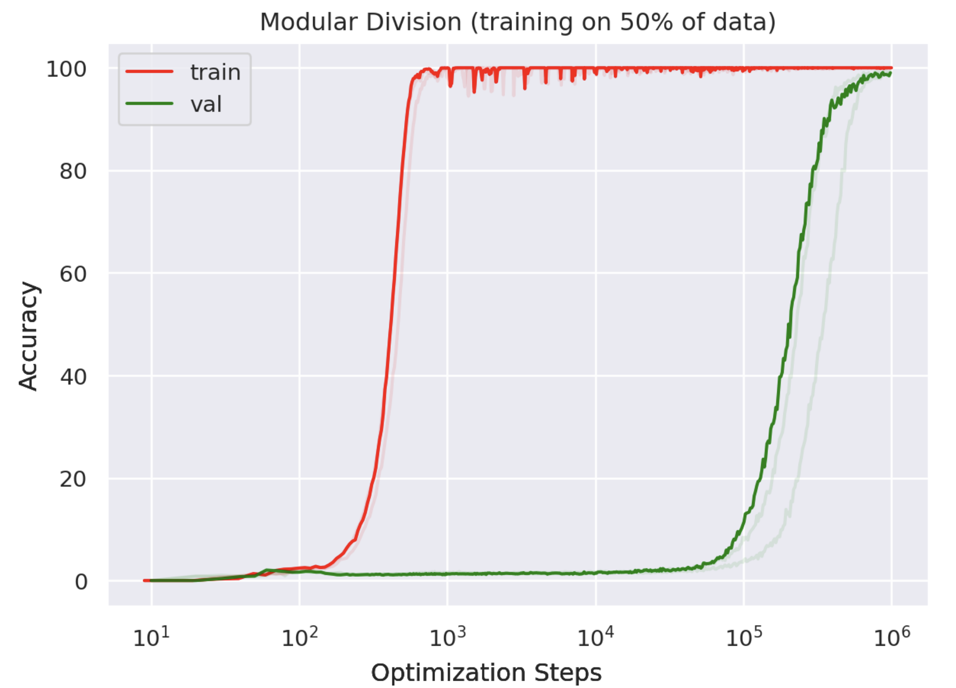Typically, when training neural networks, performance on the training dataset and validation dataset improve together early in training, and if you continue training past a certain point the model will overfit the training data and its performance on the validation data will decay. The OpenAI paper showed that the opposite can sometimes happen. Neural networks, in certain settings, can memorize their training dataset first, and then only much later "grok" the task, generalizing late in training. Here is a key figure from the original paper, showing the prototypical grokking learning curve shape:

Grokking is not a universal phenomenon in deep learning. The setup of Power et al. was fairly unusual. Most notably, they studied the problem of learning what they called "algorithmic datasets". By this they just mean learning a binary operation, usually a group operation like modular addition, multiplication, etc. Denoting such a binary operation as "$\circ$", a model takes as input $a, b$ and must output $c$, where $a \circ b = c$. They use a decoder-only transformer which takes as input the six-token seqeunce < a > < $ \circ $ > < b > < = > < ? > < eos > and produces a probability distribution over the tokens the operation is defined on ($a, b, c, \ldots$). The embeddings of $a, b, \ldots$ are trainable. The model is trained on a subset of the pairs $((a, b), c)$ of the binary operation table. Evidently, this setup exhibits some atypical learning dynamics.

This paper captured people's attention for a few reasons. First, it simply adds to the existing constellation of surprising facts about deep learning generalization (double descent being another). Second, it may give some practitioners the (probably false) hope that if their network is struggling to learn, maybe they can just keep training and the network will magically "grok" and perform well. Third, grokking is an example of an unexpected model capability gain. It seems that More is Different for AI. With large language models, for instance, it is difficult to predict how performance on downstream tasks will improve as they are scaled up – large improvements sometimes occur suddenly when models hit a certain size. In the case of grokking, neural network performance can unexpectedly improve, not as models are scaled up, but rather as they are trained for longer. These unexpected model capability gains are interesting from an AI safety perspective since they suggest that it may be difficult to anticipate the properties of future models, including their potential for harm. Understanding these phase transitions in model behavior could prove important for safety.

What should we aim to understand about grokking -- generalization, beyond overfitting, on algoritihmic datasets? Here are a few key questions:

1. "Algorithmic datasets" are weird. How do models generalize on them at all? If you point out some dogs to a human child, pretty soon they can "generalize" and identify other dogs. But if you showed a child half the entries of some binary op table, would you expect them to be able to "generalize" and fill in the other half? If the table was for something familiar like addition or multiplication, they might recognize the pattern. But our networks have no pre-existing knowledge about these operations. So it just seems bizarre that they would generalize at all. What even is the right way to fill in missing entries in a binary op table, without knowing what operation it is? Maybe the only option is to evoke Kolmogorov complexity and identify the computationally simplest operation that matches the entries that are given to you (training data)? How do neural networks solve this problem?
2. In their paper on grokking, Power et al. observed that as they reduced the size of the training dataset, the time it took before their models grokked (generalized) increased dramatically. This critical training data fraction was somewhere between 30-40% of the full table. What is behind this dependence on training data fraction.
3. Why do neural networks first memorize their training dataset and only later generalize? Why don't they generalize early, as is usually the case?

In our paper Towards Understanding Grokking: An Effective Theory of Representation Learning , we sought answers to these questions. We approach the problem via an analysis of representation learning. I don't think that we fully answer the three questions, but I do think that we present both (1) some interesting empirical observations and (2) an interesting style of theoretical analysis.

Structured Representations Associated with Generalization

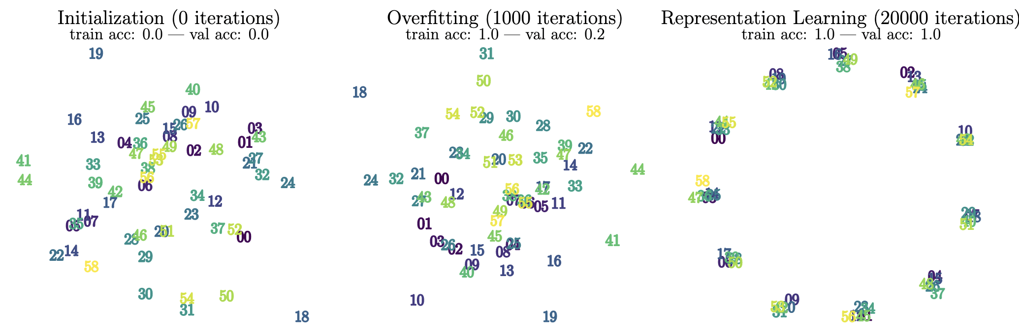
We begin with an empirical observation. With an architecture similar to what Power et al. used¹, we train on the task of modular addition ($p = 59$) and observe grokking. Across training, we do a PCA on the token embeddings and visualize their first two principal components.² See the figure below: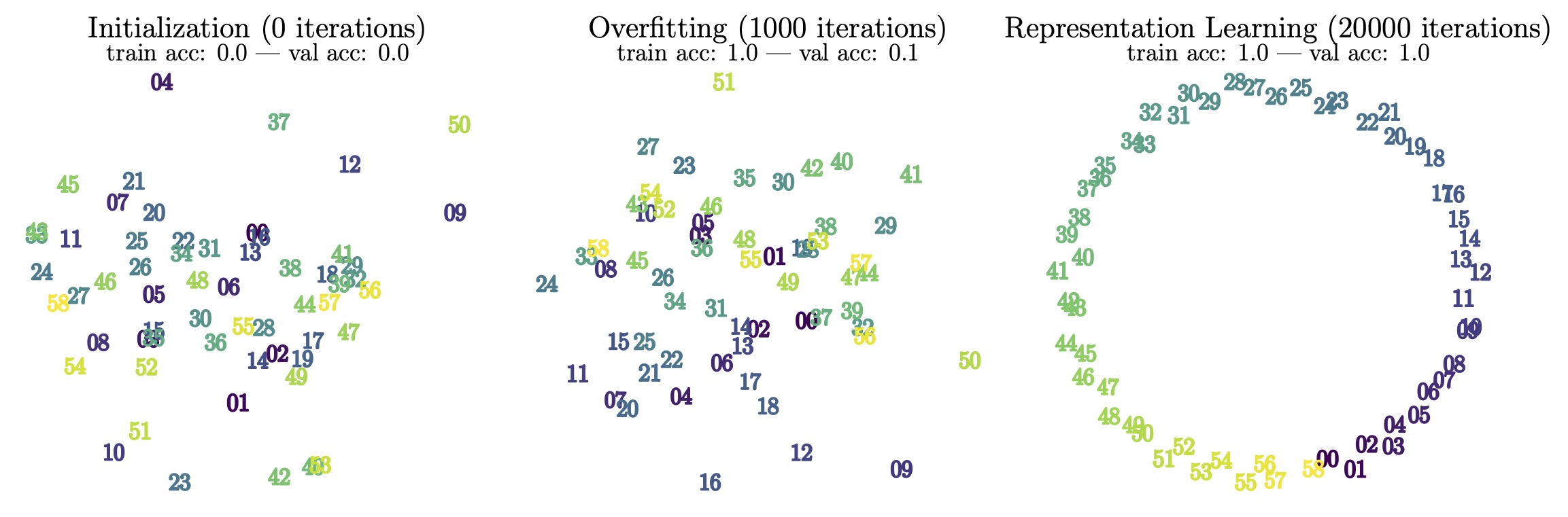


We see something interesting when we do this: generalization is associated with a distinctive ring structure in the embeddings. Furthermore, the embeddings are very precisely ordered along the ring, looping back to 0 after 58. Here is a video showing how the embeddings change throughout training:


Note that the model hits 100% validation accuracy at around step 3700. Right before this, there seems to be some quick movement where the embeddings are repelled from the center into a loose ring. At the instant when the model fully generalizes, there seems to be a global ordering of the embeddings but more locally they do not seem to be ordered very precisely. The ring becomes more precise, and the embeddings become fully ordered, if one continues training for a while. Instead of doing a PCA at each step, it is useful to visualize the embeddings along the top two components computed at the end of training.:


It appears that the two principal components at the end of training are those for which the randomly-initialized embeddings were already globally somewhat ordered. From this video, it appears that generalization occurs when the embeddings correctly order themselves additionally at the local level. If you track how "19" moves throughout training, for instance, you see that at initialization it is positioned after (counterclockwise) 20, 22, arguably 25, and on top of 23. When the network has generalized, 19 is "correctly" positioned between 18 and 20. Not all the embeddings appear to be ordered correctly at the moment of full generalization (see 4, 10, 17, 33, 42, and 44), though if one continues to train for longer they become fully ordered.

It is interesting how this circular, ordered layout resembles how we humans visualize modular addition as "clock math". However, different orderings are sometimes learned with different seeds (e.g. consecutive embeddings might be spaced about 1/4th of the circle apart instead of 1/59th), so we should be careful about drawing too much from this resemblance. What we do draw from these experiments is that there appears to be a connection between generalization and the embeddings arranging themselves in some structured way. We do not claim that this structure is fully captured by our 2-dimensional PCA plots (the fact that the network first generalizes when a few embeddings are still "out of order" suggests that other dimensions are at play, or that the PCA axes are not quite the most relevant projection), though we do find them very suggestive...

Our Theory (speculative, a bit beyond the scope of the paper)

For any given feedforward neural network, the "early layers" and the "late layers" are engaged in a kind of cooperative game. The "early layers" transform the network's input into some representation, and the "late layers" perform some computation on this representation to produce the network's output. The job of the "early layers" is to service the "late layers" with a usable representation. The job of the "late layers" is to compute the correct output from this representation -- to not bungle the good work that the "early layers" have done in giving them a workable representation!

For algorithmic datasets, we conjecture that there are special, structured representations that the "early layers" can learn which allow the "late layers" to internally implement an operation isomorphic to the "algorithmic" operation itself (modular addition, multiplication, etc.). Thus on algorithmic datasets, the setting of grokking, the reason why the network is able to generalize at all is because internally it is performing something akin to the true target operation. It is not just "fitting" the dataset, but rather its internal structure corresponds in some way to the process that generated the data.

There is a difficult coordination problem that the "early layers" and the "late layers" have to solve for this special internal operation to be learned. In particular, if the "late layers" learn much faster than the "early layers", then they will quickly fit bad, random, approximately static representations (given by the "early layers" at initialization), resulting in overfitting. On the other hand, if the "early layers" learn much faster than the "late layers", then they will quickly find (weird) representations which when thrown through the bad, random, approximately static "later layers" will produce the desired outputs (inverting the "later layers"). This will also result in overfitting.

Generalization requires that the "early layers" and "late layers" coordinate well. In the case of grokking, there is a coordination failure at first. The network learns unstructured representations and fits them. But it can't do this perfectly (the training loss is not exactly zero), giving some training signal for the "early layers" and "late layers" to work with. We suggest that the "later layers" will be less complex, and able to achieve lower loss, if they learn to perform something akin to the underlying binary operation. The reason is that, if some part of the network internally implements the binary operation, then the downstream layers need only fit $p$ representations, the operation output, instead of $\mathcal{O}(p^2)$ points, the operation inputs. Regularization schemes like weight decay, reported to be helpful in producing generalization in the original grokking paper, provide a training signal towards lower-complexity "late layers" which perform the target operation internally.

In theory, there are as many ways of arbitrarily dividing a network into "early layers" and "late layers" as there are layers in the network. For the Transformer setup, we consider the learned embeddings to be the "early layers" and the whole decoder to be the "late layers". Based on the picture presented above, we should expect that the decoder learning rate, relative to the learning rate that the embeddings are trained with, and the decoder regularization (weight decay here) should control grokking. Indeed, doing a grid search over decoder learning rate and weight decay, we find a variety of learning behaviors, with grokking occurring within a certain strip of learning rates.

A Toy Model and Effective Theory

The basic picture we've laid out is that maybe models (1) find a good representation of inputs (2) internally perform something akin to the target binary operation with these representations and (3) map the result to the desired output. It would be cool to mechanistically understand our models to check this, though we haven't done this yet. Instead, we developed a toy model capturing this basic structure and studied its properties.

We consider learning the binary operation of addition (not modulo anything -- it's not closed, so if inputs are from $0, \ldots, p-1$, outputs are from $0, \ldots, 2p-2$). Our toy model takes as input the symbols $a, b$, maps them to (trainable) embeddings $\bm{E}_a, \bm{E}_b \in \mathbb{R}^{d_{\text{in}}}$, adds these together, then maps the result to targets with an MLP decoder: $$ (a, b) \mapsto {\rm Dec}(\bm{E}_a + \bm{E}_b). $$ This kind of toy model is nice since we see that generalization comes directly from learning structured representations. In particular, if the model learns to place the embeddings $\bm{E}_0, \bm{E}_1, \bm{E}_2, \ldots, \bm{E}_{p-1}$ evenly spaced along a single line, i.e. $\bm{E}_k = \bm{v} + k \bm{w}$ for any $\bm{v}, \bm{w} \in \mathbb{R}^{d_\text{in}}$, then if the model achieves zero error on training sample $((i, j), i+j)$, it will generalize to any other sample $((m, n), m + n)$ for which $m + n = i + j$. This is because the input to the decoder will be the same for these two samples. To say it again: in this toy model, generalization comes directly from learning structured representations.

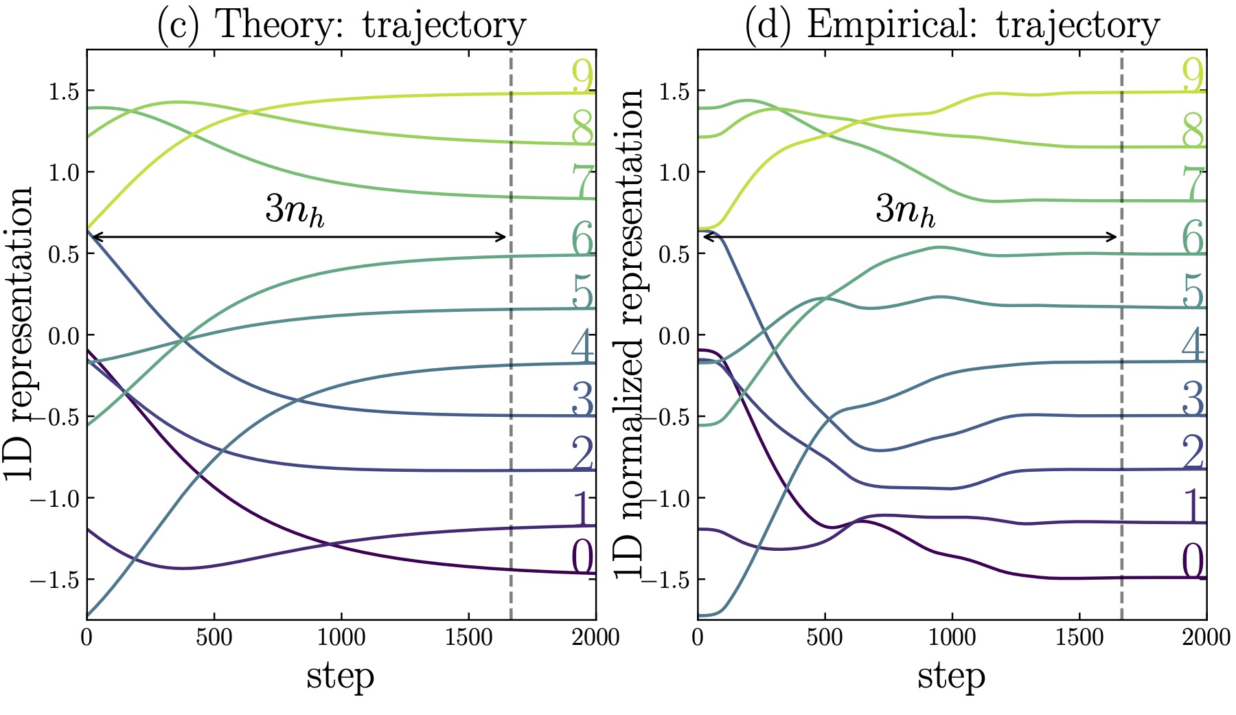
What do the learning dynamics of the embeddings $\bm{E}_{*}$ look like for this toy model? What determines whether the model learns to arrange the $\bm{E}_{*}$ along a line? We develop an effective theory for the learning dynamics of embeddings. The way that the $\bm{E}_{*}$ evolve over training, in practice, will depend on the decoder and the relative learning rate between the $\bm{E}_{*}$ and ${\rm Dec}$, as well as other optimization hyperparameters and regularization. As discussed earlier, if the decoder learning rate is much faster than the learning rate for the embeddings, the model will likely overfit to the embeddings at initialization. In the effective theory presented in this first paper, we have not incorporated any facts about the decoder into our effective theory. This means that we can't yet analytically predict how learning hyperparameters determine grokking -- we can't compute the phase diagram of learning behavior, shown above, analytically. However, our effective theory does seem to predict the dependence of grokking on the training set size, question #2 mentioned earlier.

We model the learning dynamics of the $\bm{E}_{*}$ as evolving under an effective loss $\ell_\text{eff}$. This effective loss basically measures how well/poorly the embeddings are arranged along a line. We define it as: $$ \ell_\text{eff} = \frac{1}{Z_0} \sum_{(i, j, m, n) \in P_0(D)} |(\bm{E}_i + \bm{E}_j) - (\bm{E}_m + \bm{E}_n)|^2 $$ where $Z_0 = \sum_k |\bm{E}_k|^2 $, and $P_0(D)$ is defined as: $$ P_0(D) = \{ (i, j, m, n) : (i, j), (m, n) \in D, i + j = m + n \} $$ where $D$ is the training dataset. $P_0(D)$ consists of pairs of elements in the training dataset which have the same sum. We see that if the $\bm{E}_{*}$ are evenly-spaced on a line, then $\bm{E}_i + \bm{E}_j = \bm{E}_m + \bm{E}_n$ for $(i, j, m, n) \in P_0(D)$, and thus $\ell_\text{eff} = 0$. The learning dynamics under this loss are: $$ \frac{d\bm{E}_i}{dt} = -\eta \frac{\partial \ell_\text{eff}}{\partial \bm{E}_i} $$ First, we find that, despite all simplifications and assumptions of the effective theory, that the dynamics of the $\bm{E}_{*}$ (or rather normalized versions of them) under the effective loss seems fairly similar to the dynamics under real training with a decoder. Below we show a comparison of the two dynamics for 1D embeddings $d_\text{in} = 1$


Second, when we vary the size of the training dataset $D$, we find that the effective theory predicts the likelihood that the model will generalize -- that it will learn to arrange the embeddings along a line -- decreases rapidly once you go below a train set fraction of 0.4:


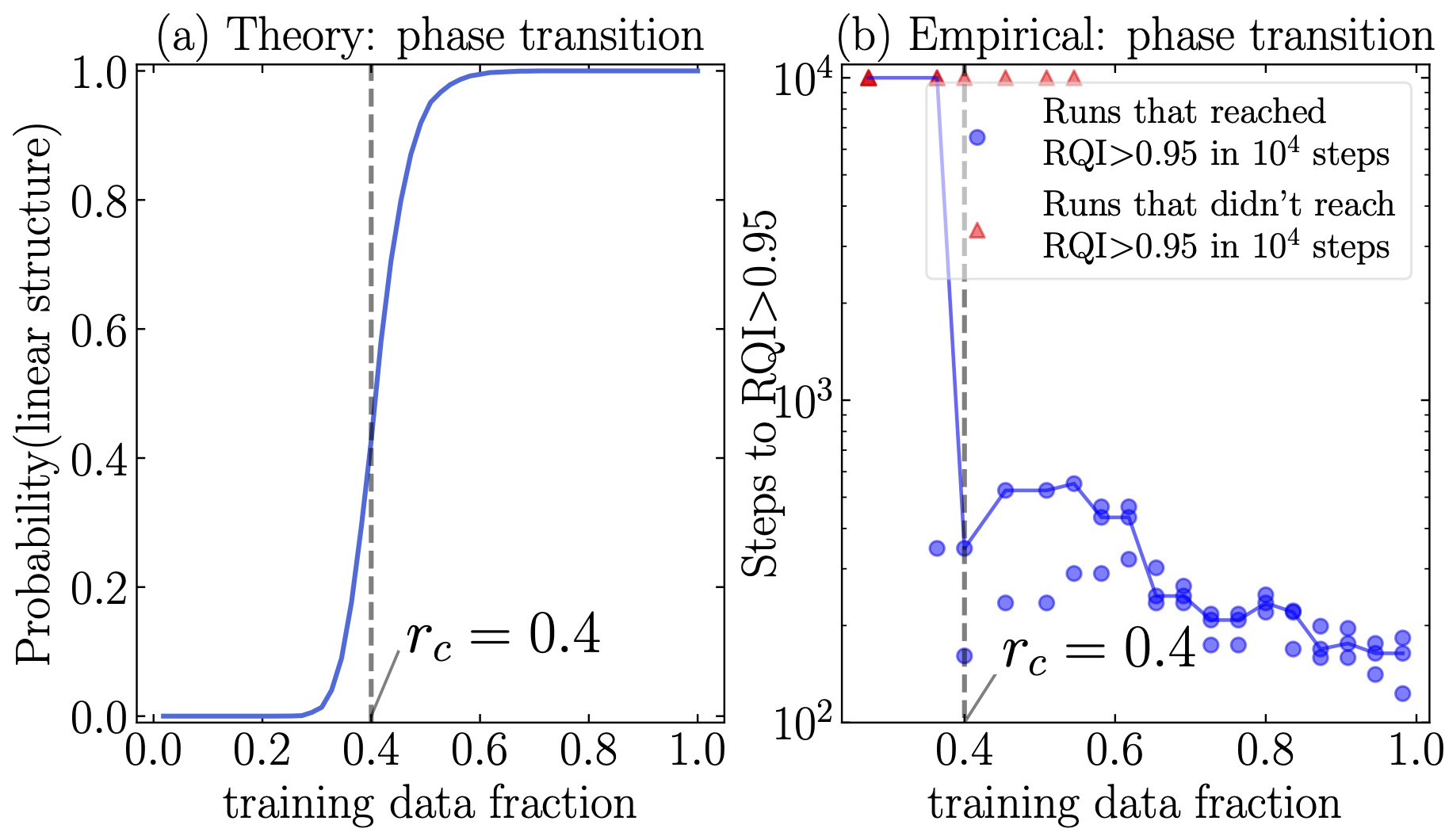
Admittedly, what we are more interested in is the time that it takes to generalize, not the probability of generalizing at all. I won't give the full argument here, but from our effective theory one can perform an analysis of the eigenvalues of a certain matrix $H$ which governs the dynamics, and find that the first nonzero eigenvalue $\lambda_3$ corresponds to the speed at which learning happens, and that $\lambda_3$ is quite sensitive to the train set fraction.

Related Work

Some writers had made informal posts with conjectures about grokking before our paper. Beren Millidge had an interesting post where he discussed learning, during overfitting, as a random walk on an "optimal manifold" in parameter space, which eventually hits a region which generalizes. He discusses weight decay as a prior, when one views SGD as MCMC, and makes a connection to Solomonoff induction. Rohin Shah also made some conjectures in the Alignment Newsletter about how functions which memorize will likely be more complicated and therefore provide worse loss for a given level of expressivitiy than functions which generalize. Then if the training during overfitting is mostly a random walk, once it finds a function which generalizes it will stay there because the loss will be lower.

A more involved explanation was offered by Quintin Pope in his LessWrong post Hypothesis: gradient descent prefers general circuits. He envisions the training process as one in which "shallow" circuits are slowly unified into more "general" circuits which generalize. I find this description to be pretty intuitively appealing, though it has not been backed up yet by a deep mechanistic circuits-style analysis of real networks. Perhaps our observations about structure emerging in the PCA of embeddings will be useful in identifying these general circuits. As discussed earlier, a lot is involved in a network learning a general circuit, one which effectively implements the target operation. A necessary condition seems to be that good representations are learned, and we have modeled this aspect of learning a general circuit, of representation learning, with a simplified effective theory. This allowed us to analytically study the effect of the training data fraction on learning. But we do not yet have a full account of how these general circuits are formed.

Taking Stock

In terms of our original three questions about grokking, I think that we have a partial answer to (1), a reasonable answer to (2), and a partial answer to (3).

In terms of question (1), about why generalization happens at all, I think our observations about structured representations being associated with generalization suggests that the network is doing something very clever internally. It is probably doing something like internally implementing the target operation (otherwise how would it generalize?), but we don't yet understand mechanistically how it does this. By the way, embeddings arranged on a ring seem pretty typical for many tasks, but the order changes. Here is non-modular addition, instead of mod 59:


Interestingly, within each bundle on the ring are numbers belonging to the same "parallelogram". At one o'clock we find the embeddings for 2, 13, 24, 35, 46, and 57, for which 2 + 57 = 13 + 46 = 24 + 35. Pretty neat.

For question (2), we studied a toy model of grokking where the relationship between structured representations and generalization is clear. We modeled the learning dynamics of these representations under an effective loss, and found that this model captures the dependence on training set size pretty well.

For question (3), we have some heuristic arguments about learning speed between different parts of a network, but I don't feel that we fully understand why grokking appears on algorithmic datasets and not on more standard tasks. It likely has something to do with how a particularly special circuit must be learned for generalization to occur on algorithmic datasets...

Always more to think about!

Footnotes

<sup>1. Our transformers have a sequence length of just two, "< a > < b >", rather than having a longer sequence length in which all the other tokens are constant for all samples.↩
2. The original paper on grokking from Power et al. showed a visualization of embeddings with t-SNE, but we find the PCA projections to be more interesting. We also track how structure in the embeddings changes over training, whereas they just showed embeddings of the trained network.↩</sup>